Interactive model: two users on the same radio resource
Interactive · Radio technology explained
Explore 5G beamforming
Two phones share the transmit power. The switches show the relationship between desired signal and mutual interference.
User A
- Desired signal
- –
- Interference from B
- –
User B
- Desired signal
- –
- Interference from A
- –
Desired signal: same position, both switches off = 100 %. Interference: the other stream’s power relative to the current desired signal.
Show angles and outside-region levels
How the model works · Assumptions and limits
The visualisation
The 64 element positions form a schematic 8 × 8 array at 3.6 GHz. Each shape shows the directions in which one stream radiates more or less strongly. Each displayed beam is individually normalised.
What the numbers compare
With two users, each stream receives half a fixed total power. The desired signal is compared with the same geometry and both switches off. Interference is relative to the current desired signal at each phone.
Simplifying assumptions
The model uses ideal line-of-sight links and known radio directions. Multipath, measurement errors, noise, neighbouring cells and polarisation are outside the calculation. Data rates and real-site coverage would require further modelling.
The 21 test directions are freely chosen examples illustrating CSI-RS-based measurement. The sequence is slowed down for observation. In this example, the same direction is used for measurement and data transmission.
Element positions, radio chains and data streams describe different things. The 8 × 8 model is independent of any particular real-world antenna hardware configuration.
- Ericsson: Massive MIMO for superior network performance
- Ericsson: Broad beamforming technology in 5G Massive MIMO
- 3GPP TR 38.901 V19.5.0, clause 7.3.0, Table 7.3-1, and clause 7.3.1
- MathWorks: Introduction to Null Steering
- MathWorks: lcmvweights
- 3GPP TS 38.211 V19.5.0
- 3GPP TS 38.213 V19.5.0
- 3GPP TS 38.214 V19.5.0
What do the percentages mean?
Desired signal: The reference uses both switches off at the same phone position, with the same beam-selection mode and transmit power. A value of 100 % matches that reference; 50 % means half its desired-signal power. Movement recalculates the reference at the new position.
Interference: Here the reference is the current desired signal at the same phone. At A, the display evaluates the unwanted stream intended for B; at B, it evaluates the stream intended for A. A value of 10 % means the unwanted beam arrives at one tenth of the desired power. At 100 %, both are equally strong. “< 0.01 %” is effectively zero relative interference in this ideal model.
An example: Suppose the desired power is 100 arbitrary units with both switches off. After switching, 50 units remain, and 5 units arrive from the other beam. The display then shows Desired signal: 50 % and Interference: 10 % because 5 is one tenth of the current 50.
The two indicators use different reference quantities. They describe relative received powers; connection speed and packet loss require additional information.
How does suppression work?
Many small antenna elements jointly transmit the stream for A. Their amplitudes and phases are adjusted so the contributions reinforce at A and cancel at B, like a crest meeting a trough. This creates a null for A’s stream at B. The process is reversed for B’s stream. Each phone can then receive its own stream with less mutual interference.
What does sidelobe control do?
Additional weighting reduces the total radiation in selected unwanted directions while preserving enabled nulls at the phones. This can weaken the desired signal and reshape the main lobe. The outside-region indicator evaluates a chosen angular region, which may include main-lobe skirts. It shows the estimated peak within that region; the optimisation does not impose a global peak ceiling.
Why can the desired signal become weaker?
The antenna must deliver power to the intended phone while placing a null at the other one. Meeting both goals can reduce reinforcement at the intended phone. Transmit power remains fixed, while the directions of reinforcement and cancellation change. A weaker desired signal can still provide a better connection when interference falls enough.
In grid mode, the desired signal can also increase: the reshaped beam may align with the phone better than the coarse initial direction.
What is simplified here?
Real 5G networks use reference signals and, depending on the procedure, feedback to estimate radio channels. The data view assumes perfectly known directions. “Find a beam” illustrates a simplified sequence of reference signals, measurements and feedback. Measurement errors, reflections and protocol timing remain outside the model.
The 8 × 8 element positions, 21 example directions and equal power split between users are chosen assumptions. A real antenna’s radio-chain count depends on its hardware. The percentages are relative comparisons within this model.
Each displayed beam is normalised individually; the numbers provide the power comparison. Exact channel knowledge enables the ideal nulls shown here. Real networks generally retain some residual interference. Data-rate prediction would require further modelling.
Massive MIMO antennas differ from conventional mobile network antennas in their many controllable transmit and receive chains and the associated signal processing. In 5G networks, they are mainly used in the mid-band, for example at 3.6 GHz. Systems also exist for lower frequencies and for millimetre-wave bands such as 26 GHz. With Massive MIMO and beamforming, a 5G base station can serve several devices, such as smartphones, at the same time on the same frequencies, increasing spectral efficiency. It shapes the radiation pattern by changing how the signals from its antenna elements combine in space. The aim is a strong desired signal at each receiver and as little interference as possible to other devices. Beamforming and Massive MIMO provide the spatial degrees of freedom needed to do this.[1]
Two phones make the relationship particularly clear. When the antenna simply reinforces the desired directions, part of each signal also reaches the other phone. Carefully calculated antenna weights can reduce this unwanted contribution. The interactive model shows how the radiation patterns and relative received powers change in the process.
The starting view shows two phones in front of an 8 × 8 array operating at 3.6 GHz. The blue and orange beams carry two independent data streams. Both use the same time and frequency resource, and each receives half the model’s fixed total transmit power. This illustrates multi-user MIMO, or MU-MIMO: spatial processing helps separate simultaneous transmissions.
In the “Two users” experiment, the position slider changes the arrangement of the phones. “Start walking” begins the run at 0 percent. After a pause, “Continue walking” resumes movement. “Reset” stops the animation and returns the position to 0 percent. “Reset view” also restores the original viewing angle. “Suppress interference” adds a null for each data stream at the other phone. “Control sidelobes” further changes the weights to reduce radiation outside the intended direction. Separate result panels show the effects for A and B.
The “Track a beam” experiment reduces the scene to one phone. The transmit direction follows its movement, making the electronic steering of the radiation pattern visible. “Beam selection and user settings” switches between an ideally tracked direction and a choice of 21 fixed example directions. The limited grid shows how a selected beam can deviate from the best alignment between grid directions.
In “Find a beam”, measurement controls replace the movement settings. After phone A or B is selected, the sequence moves through reference signals, comparison, feedback and a data beam. “Next” and “Back” advance through the steps manually; “Start sequence” plays a slow animation. Dragging or the arrow keys rotate the camera. “Top view” helps compare phone directions, while “Antenna array” shows the element arrangement. On a smartphone, “Rotate by touch” switches between camera rotation and scrolling over the scene.
How many antenna elements form a beam?
An electronically formed beam combines the contributions of several antenna elements. A simple array can contain as few as two elements; Massive MIMO antennas use many elements working together. The number depends on the antenna design and the group of elements used. At the same wavelength, a larger effective antenna aperture allows a narrower main lobe. In real antennas, several elements may form a jointly controlled sub-array.[1]
The interactive model uses an array of 8 × 8, or 64 element positions. The blue beam for user A and the orange beam for user B each use the entire array, with their own phase and amplitude weights. At every element position, the appropriately weighted contributions of both data streams are added together. The same array thus forms two different radiation patterns at the same time.
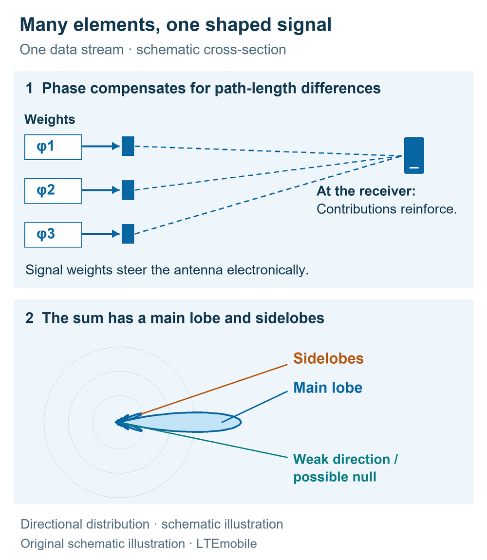
Each element in an antenna array radiates an electromagnetic wave. The contributions travel different distances before arriving at the receiver. The base station adjusts their phase, meaning their relative position within the oscillation cycle. This allows the contributions to reinforce one another in a desired direction. In other directions they combine more weakly or partly cancel. Their amplitudes also determine how strongly the individual elements contribute to the sum.
The amplitude and phase weights together form the precoder. Changing them changes the main lobe, sidelobes and possible nulls in the radiation pattern. The main lobe is the region of strongest radiation; sidelobes are additional, weaker peaks. A null is a direction with very low power. The principle also works in reception: the antenna signals are combined to reinforce a desired received signal.
What desired signal and interference mean in the model
For each phone, “Desired signal” shows the power of its intended data stream relative to a reference. The same location, the same beam-selection mode and both switches off define 100 percent. The reference is recalculated at each position. It therefore shows how signal shaping affects reception at that location. Comparing absolute received powers between locations would require a different reference.
The “Interference” indicator divides the unwanted stream’s power arriving at the phone by its current desired-signal power. For example, 40 percent means that the unwanted power is 0.4 times the desired power. This figure excludes noise and neighbouring cells. A complete measure of signal quality would also account for all interference and noise through the signal-to-interference-plus-noise ratio, or SINR.
The numerical example uses a position of 78 percent along the path, two users and direction tracking. With both switches off, mutual interference is about 41.5 percent of the desired signal at each phone. “Suppress interference” reduces it to below 0.01 percent in the ideal model. At the same time, the desired signal falls to about 58.5 percent of its reference. Some of the available spatial degrees of freedom are now being used to place a null at the other receiver.
With sidelobe control also enabled, the desired signals at this position are about 38 to 39 percent of their reference values. The additional shaping also changes gain towards the intended phone. The example shows the trade-off between concentrating power and suppressing unwanted radiation. The resulting data rate also depends on SINR, modulation, coding, bandwidth and the number of simultaneously usable streams.
Each displayed beam shape is normalised to its own maximum. Its extent shows the directional distribution. The numbers below the scene provide the power comparison. The shape has no distance scale and does not define a coverage boundary.
Beamforming, Massive MIMO and data streams
Massive MIMO combines a large number of controllable antenna branches with the associated signal processing. This provides many degrees of freedom for concentrating signals, managing interference and spatially separating several data streams. Beamforming describes the shaping of the transmit or receive response. Spatial multiplexing describes the parallel transmission of independent data streams on the same time and frequency resource.[1]
In single-user MIMO, one device receives several data streams, also called layers. The radio channel and receiver must provide enough distinguishable transmission paths. Different polarisations and multipath propagation can help separate them. In multi-user MIMO, the simultaneous layers go to different devices. The model illustrates this second case, with exactly one stream per phone. Real networks can combine both techniques.[1]
The base station needs suitable weights for each stream. In the two-user model, this creates two different radiation patterns from the same array. Successful simultaneous transmission requires sufficiently different radio channels. Similar channels are harder to separate; serving the devices at different times or on different frequency resources may then be more effective. The network scheduler makes this selection.
Four different quantities help explain antenna specifications:
| Quantity | Meaning |
|---|---|
| Antenna element | A physical radiating element in the array. Several elements may be controlled together. |
| Radio chain | An electronic transmit or receive branch. Its mapping to antenna elements depends on the hardware design. |
| Logical antenna port | A standardised association of signals with inferable channel properties, providing a reference for channel estimation and reference signals. |
| Layer / data stream | A spatially transmitted part of the user data. The usable number depends on the channel, device and network configuration, among other factors. |
The 3GPP specification defines an antenna port through the channel properties of its signals. A designation such as “64T64R” refers to the transmit and receive branches of a particular antenna system. Assessing a smartphone or 5G router also requires its supported bands and MIMO configurations. The principles of spatial multiplexing already apply to LTE Advanced.[2]
How the network finds a suitable beam
The process starts with finding a cell. In 5G, synchronisation signals and the physical broadcast channel are carried in the SS/PBCH block, often called an SSB. A base station can transmit these blocks in different directions. The device uses them to obtain synchronisation and information for the subsequent access procedure. TS 38.213 describes the possible SS/PBCH-block positions; these serve a different role from the data beams used later.[3]
The network configures additional reference signals for a more detailed assessment of the radio channel. In the downlink, CSI-RS—Channel State Information Reference Signals—play an important role. The phone measures the configured resources and provides the requested reports. The base station can use these, together with other channel information, to determine a suitable transmission. In the uplink, SRS—Sounding Reference Signals—are among the signals available for measurement by the base station.[2]
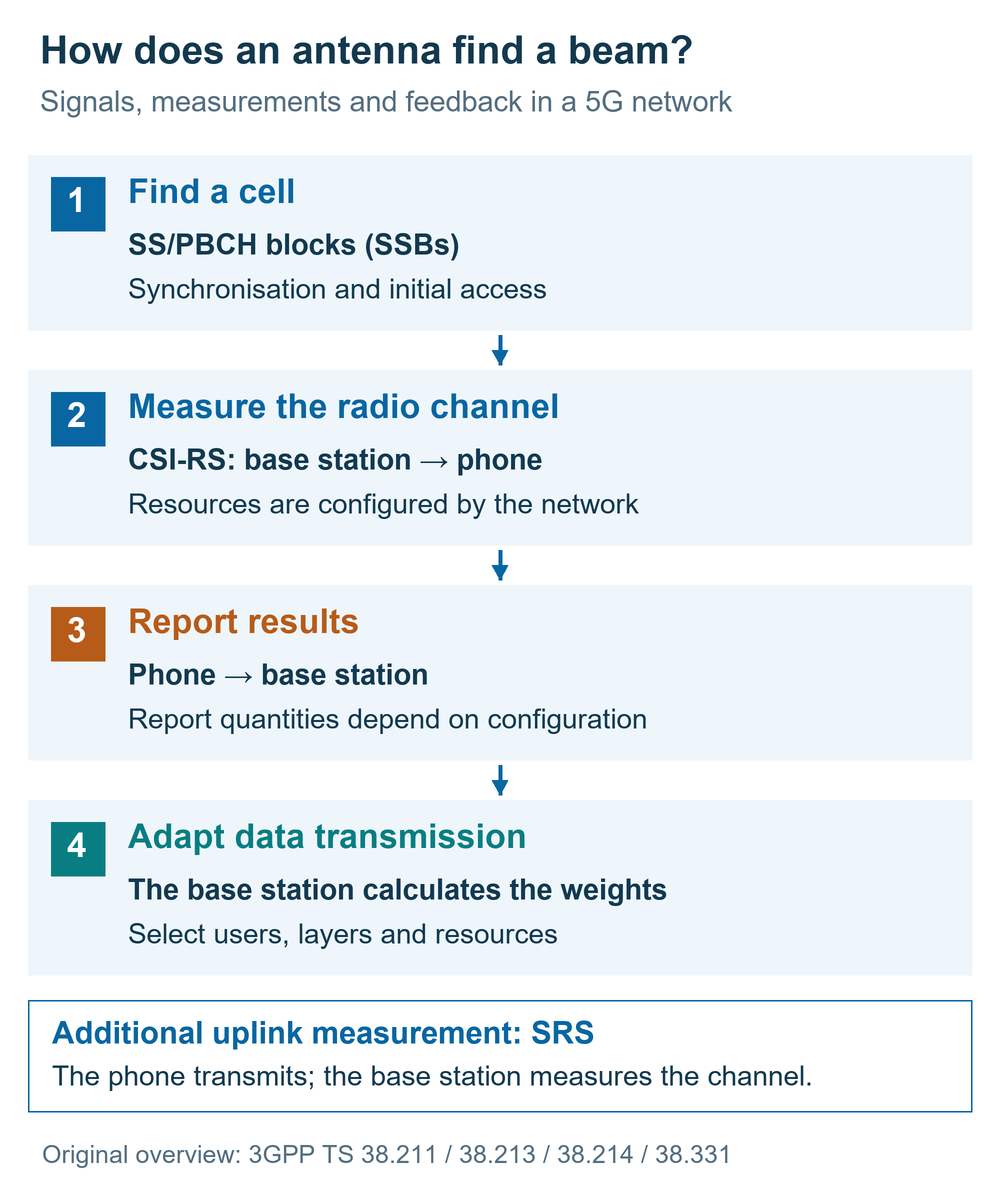
The content of a report depends on its configuration. A CRI identifies a selected CSI-RS resource. The RI indicates a recommended transmission rank, or number of layers. The PMI identifies a precoder from an agreed codebook; the CQI describes the estimated channel quality for data transmission under the specified assumptions. Other configurations request, for example, a resource index and a received-power measurement. TS 38.214 specifies which quantities are reported together.[4]
Using TCI states, the network can also signal relationships between reference signals and the channel properties used for reception. With QCL-TypeD, these include spatial receive properties, giving the device a reference for its receive configuration. TS 38.331 contains the corresponding configuration elements, including CSI-ReportConfig and TCI-State.[4][5]
The “Find a beam” experiment extracts the sequence measure, compare, report, transmit from this process. It tests 21 freely chosen directions at equal test power and selects the direction with the highest calculated received power. In this example, the same direction is used directly for the data beam. Real networks may shape measurement and data beams differently and use further information in the decision. The sequence illustrates the principle of beam-related CSI-RS measurements; the grid, feedback representation and timing are choices made for this learning model.
Model assumptions: what is calculated
The array has eight by eight element positions, spaced half a wavelength apart. At the fixed frequency of 3.6 GHz, this is approximately 4.2 centimetres. The relative element response uses the angular dependence in TR 38.901, Table 7.3-1, with a 65-degree parameter in both principal cuts and a 30 dB limit on element attenuation. The constant maximum gain in that table is factored out for these relative comparisons.[6]
For each direction, the model adds the complex element contributions with their respective phases. It assumes ideal line-of-sight links and precisely known channel directions. The drawn crossed dipoles illustrate the antenna structure; the calculation itself remains scalar. Polarisation differences, multipath propagation, shadowing, noise, neighbouring cells and measurement errors are outside the calculation.
Null steering calculates weights that ideally cancel the unwanted stream in the actual direction of the other phone. Sidelobe control adds a separate optimisation to reduce radiation in a selected outer angular region. Both procedures can freely adjust amplitude and phase. This gives them more flexibility than some real hardware arrangements with grouped elements or restricted control ranges.
Under “Show angles and outside-region levels”, the outside-region level applies to a chosen region starting 14 degrees away from each beam’s initial direction. It may also include main-lobe skirts. The optimisation reduces weighted power over its outer-region design grid, while the indicator reports the numerically estimated peak in that region. The 14-degree boundary and optimisation method are model choices.
Movement and beam-selection animations are slowed down for observation. Protocol timing, measurement intervals and network response times are outside their scope. Resource scheduling, rank selection, coding and data packets are also outside the simulation. TR 38.901 supplies a building block for the element response; its full radio-channel model is not implemented here. The technical specifications describe the real signals and procedures, while the learning model uses its own implementation of weight optimisation.
What spatial processing does in a mobile network
A larger effective antenna aperture generally allows a narrower directional response at the same frequency. Frequency, element spacing, element response and weights jointly determine the radiation pattern. Reflection and diffraction add further paths in a real radio channel. These paths change the weights that produce a favourable combination at the receiver; distinguishable paths can also support several MIMO layers.
Massive MIMO uses these spatial properties to make better use of the available radio resources. Whether this provides more desired-signal power, a better interference situation or additional parallel transmissions depends on the channel and the simultaneously active devices. The two-user example makes part of this decision visible: greater suppression of mutual interference also changes the desired signal. A real network assesses these effects together with its resource and transmission planning.
The guide to 5G frequencies and bands explains the available spectrum. The article on 5G range at different frequencies adds the propagation conditions. The interactive antenna view explores the shape of an individual antenna pattern. The article on 5G SA and NSA explains how the radio and core networks work together.
Sources and technical references
The technical references were checked against the supplied original 3GPP documents. The cited versions date from September 2026. Both explanatory graphics and the interactive model are original LTEmobile illustrations; the standards documents are linked as sources.
- Ericsson: Massive MIMO for superior network performance. Sections “Multi-antenna techniques”, “Beamforming”, “Null-forming”, “MIMO techniques”, “Antenna array structure” and “Evolution of Massive MIMO”; explanation of beamforming, SU-MIMO, MU-MIMO, array structure and frequency ranges.
- 3GPP TS 38.211 V19.5.0. Clauses 4.4.1 (antenna ports), 6.4.1.4 (SRS), 7.3.1.3 (layer mapping) and 7.4.1.5 (CSI-RS).
- 3GPP TS 38.213 V19.5.0. Clause 4.1: cell search and SS/PBCH blocks.
- 3GPP TS 38.214 V19.5.0. Clauses 5.1.5 (TCI/QCL), 5.2.1.4.2 (report quantities), 5.2.1.4.3 (L1-RSRP reporting) and 5.2.2.2 (PMI/codebooks).
- 3GPP TS 38.331 V19.4.0. Clause 6.3.2, including CSI-MeasConfig, CSI-ReportConfig and TCI-State.
- 3GPP TR 38.901 V19.5.0. Clause 7.3.0, Table 7.3-1 (element response), and clause 7.3.1 (antenna-port mapping and complex weights).